In Chapter 9 of The Domino Effect, we examined the production economics for an important shale play, one with multi-commodity economics: the Wolfcamp play in the Permian Basin of West Texas. Prior to the crude price crash in late 2014, Wolfcamp producers enjoyed high returns on their typical wells primarily due to the triple-play nature of most Permian wells – yielding not just crude oil but also natural gas and natural gas liquids.  Over a year later in Q4 2015, production from the Wolfcamp was still increasing, in part due to the relatively attractive rates of return on these wells.

To demonstrate how these returns are calculated, Chapter 9 walked through the inputs required for The Domino Effect Production Economics Model for a representative Wolfcamp well.  However, the book did not get into the mechanics of using the model.  In this Extra Content segment, we explore the spreadsheet model itself and provide the opportunity to download the Excel model file.  Note that the input values described below are defined and quantified in Chapter 9, based on a premise of “half-cycle” economics.  Half-cycle economics means the calculations only consider the cost of drilling and completing the well, not the cost of exploration activities or acquiring the lease. 

Before getting started with the description of model inputs, you need to download The Domino Effect Production Economics Model. 

If you have trouble downloading the file (usually some firewall issue), then let us know at info@thedominoeffect.com.

Model Inputs

Drilling and Completion (Capital) Costs and Other Model-Wide Variables.  Figure #1 below is a screenshot of the model input section for drilling and completion costs and a few other key variables.  Our color convention is that input fields are in blue, output results are in green and yellow cells are descriptions and labels. We also labeled input columns (letters) and rows (numbers) on the table in Excel format to help you find the right cell. The cell references that we use in this description match the cell references in the spreadsheet. Do not attempt to change cells that are not blue; the rest of the cells are calculated by the model.

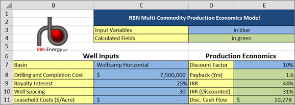
Figure 1 – Well Inputs

Drilling and Completion Cost: (cell C8) is the total cost of drilling and completion for our representative Wolfcamp well of $7.5 million.

Royalty Interest: (cell C9). This is an agreed upon percentage of the gross production revenue paid to the owner of the mineral rights. The royalty interest varies according to lease terms but is trending at about 25 percent in the Permian.

Well Spacing: (cell C10). The number of acres per lease well.  30 acres is used as a default in the model, but the number of acres per well continues to decrease. Since we are calculating half-cycle economics for this well, well spacing is not used in the calculations.

Leasehold Costs ($/Acre): (cell C11). This is the input value for the ‘bonus’ cost of a lease on a dollars per acre basis.  Since we are calculating half-cycle economics, this variable is set to zero.

Discount Factor:  (cell E7) The discount factor is the interest rate used to calculate the cumulative Discounted Cash Flow for all three commodities: oil, natural gas and NGLs in column E. The sum of the discounted cash flows is the net present value (NPV). The model calculates the value of the discount factor when the NPV is zero as the internal rate of return (IRR), or discounted cash flow rate of return: (cell E10). The discount factor could be as simple as a published interest rate but typically represents a company’s internal cost of capital. We set the default discount rate in the model to 10% because operators often calculate a well’s break-even price on a before tax basis using a flat 10% discount rate. This facilitates an “apples to apples” comparison both between wells and across companies.

We will come back to the results cells in green following our discussion of the remaining input cells.

TAXES, OPERATING COSTS, AND ESCALATORS

Figure 2 below shows the input cells for product specific costs.

Production Taxes: Oil and gas each have a different assumed production tax: 4.5% (cell L12) for oil and 7.5% (cell X12) for natural gas. The production tax is levied on the final sale price of the oil and gas at the wellhead. Usually production taxes apply to net revenue less royalty payments.

Operating Costs (called Incremental cost in the Model): Variable costs associated with the production of oil (cell L10); gas (cell X11); and the processing cost for NGL’s (cell AJ11) Set at $10/bbl for oil and $1/Mcf for gas, and 30 cents/Mcf for NGLs.

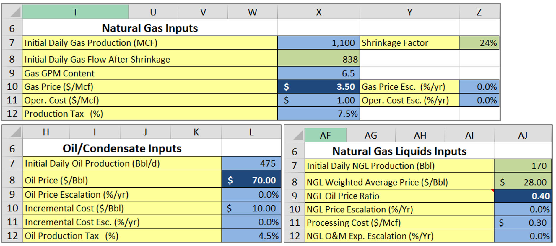
Figure 2 – Commodity Specific Inputs

Incremental Cost (operating expenses) Esc. (%/yr): (cell L11). This is the expected annual escalator for oil-related variable costs (see Operating Costs above). In this version of our model we kept both prices and costs constant, so no value is assigned to this cell.

Operating Cost Esc. (%/yr): (cell Z11). This is the expected annual escalator for gas-related operating costs. As indicated above, our assumption for this well analysis is constant prices and costs so no default value is assigned.

NGL O&M Exp. Escalation (processing cost) (%/Yr): (cell AJ12):  This is the expected annual escalator for NGL operating and maintenance costs. Same assumption as above.

IP RATES, DECLINE RATES AND GPM

Initial Production [Oil/Gas/NGL]: (cell L7 for oil; X7 for gas; AJ7 for NGLs). This is the first year’s daily production rate (measuring volume in Bb/d for oil and NGLs, Mcf/d for gas). Production is multiplied by the assumed commodity price to calculate gross revenue. After the first year, production is calculated using the production decline rate (see Decline Rate below). For our representative well, the initial daily production is 475 bbl/d for oil and 1,100 Mcf/d for gas. We will demonstrate how the NGL initial production is modeled in the Calculated Results section below.

Gas GPM content: (cell X9) is the gallons per MCF, or NGL content of the inlet gas stream at the processing plant.  Our representative well yields 6.5 GPM, which is within the range of typical horizontal Wolfcamp wells in the Midland Basin.

Decline Rate: (cells H18-27 for oil; T18-27 for gas) The production decline rate in the model, starting at 55% for first year in the table below (column H in Figure 3 shows the decline rate for oil) is input as a variable for the first 10 years of production then remains unchanged after year 10 (5%) through the remaining life of the well. The numbers input into the decline rate are variable fields that can be calculated using a number of methods outlined above. The default values set in the model are based on a simple percent annual decline curve.  In our representative well we have assumed the decline rates for oil, gas and NGLs are the same in each model year.

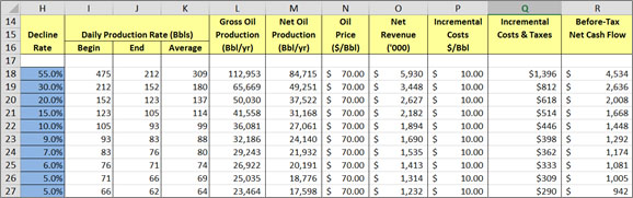
Figure 3 – Annual Crude Revenue

 

Oil Price ($/Bbl) and Gas Price ($/MCF): (cell L8 and cell X10, respectively). These are the netback prices for oil and gas at the wellhead. Netback price is the selling price less transportation costs. At the time this model was created, we used a $70/Bbl oil price and a $3.50/Mcf gas price. The NGL Price ($/Bbl) in cell AJ8 is calculated as a ratio of the Oil Price (cell L8) using the input ratio value in cell AJ9. The default ratio in cell AJ9 is derived from the current value of NGL’s relative to crude.

Oil Price Escalation (%/yr): (cell L9). This input is the expected annual (d) escalation of the Oil Price ($/Bbl). This factor is multiplied by the Oil Price ($/Bbl) (cell L8) to calculate a new oil price every year (cells N18 through N42). Since we have assumed constant prices and production costs, this factor is zero in the default model.

Gas Price Esc. (%/yr): (cell Z10). This input is the expected annual (d)escalation of the netback price of natural gas in the Gas Price ($/MCF) variable. This factor is multiplied by the Gas Price ($/MCF) in (cell X8) to calculate a new gas price every year (cells Z18 through Z42). As indicated above, the factor defaults to zero for our representative well.

NGL Price Escalation (%/yr): (cell AJ10) NGL prices are tied to oil prices in the default model, so this value is set to zero. 

The model computes a revenue, operating cost and before-tax (income tax) net cash flow for each of the three hydrocarbon commodities. Crude oil production volume is based on the IP rate and decline rate for crude, smoothed using the Arps model described above.

NGL VOLUMES AND SHRINKAGE

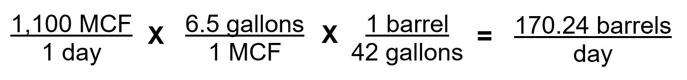
The IP rate and decline curve inputs for natural gas are used to compute gross gas production.  Then the liquids content of the gas (GPM) is used to compute the NGL volumes.  Using the 6.5 GPM value in our model and the 1,100 Mcf/d IP rate for gas, the initial production rate for NGLs is then calculated as 1100*6.5/42=170.24.  Of course 42 is the number of gallons in a barrel.

When NGLs are extracted in a processing plant, the volume of gas remaining is naturally going to be less than the original wellhead production.  This “shrinkage” is computed by the model based on a typical mix of NGL products in the NGL barrel: 50% ethane, 27% propane, 8% normal butane, 6% isobutane and 9% natural gasoline.   This simplified model does not provide the ability to change this mix of NGL products.

To calculate the shrinkage we multiply the Initial Gas Production (cell X7) by the computed Shrinkage Factor (cell Z7) then subtract the resulting shrinkage from the Initial Gas Production to arrive at Initial Daily Gas Flow after shrinkage (cell X8).  For example:

1100 MCF/d x 24% shrink = 262 MCF/d
1100 MCF/d - 262 MCF/d = 838 MCF/d Initial Daily Gas Flow after shrinkage

OIL AND GAS PRICES

The prices are input as noted for oil and gas, but calculated for NGLs in cell AJ8 using the simple .4 ratio discussed under NGL Price ($/Bbl) above.

ANNUAL CASH FLOWS, CUMULATIVE CASH FLOW, DISCOUNTED CASH FLOW

Cash flows for each of the three hydrocarbon products are summed with total investment costs to yield annual cash flows and cumulative cash flows. As indicated in Figure 4, based on the input discount factor of 10%, discounted cash flows are then computed in Column E.

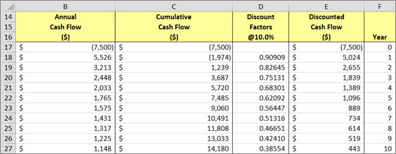
Figure 4 – Cash Flows

PAYBACK AND INTERNAL RATE OF RETURN

The discounted cash flow (DCF) of $10.3 million for this well, shown in cell E11 (Figure 1), is the sum of the discounted cash flows in column E. The sum of the discounted cash flows is also known as the Net Present Value (NPV). The discounted cash flows are the cumulative pre-tax cash flows per year summed for all three commodities in column C, with the $7.5 million well cost netted out, multiplied by the discount factor in column D.

Well Payback, shown in cell E8 (Figure 1), quantifies the amount of time it takes to recover the well investment (1.6 years for our representative well). This is because first two years annual cash flows, of $5.5 million and $3.2 million respectively, exceed well cost. (cells B18 & B19).

The model computes two Internal Rates of Return, with one considering the cost of capital in the calculation and the other ignoring cost of capital.    Both returns are calculated using the Excel function =IRR().   The Internal Rate of Return (cell E9) is the rate which discounts the series of before tax net cash flows in cells B17 to B42 to zero.  Using this calculation, the value for our representative Wolfcamp well (at $70/bbl oil and $3.50 gas) is 44%.  The Internal Rate of Return - Discounted (cell E10) is the rate which discounts the series of before tax discounted net cash flows in cells E17 to E42 to zero.  The calculated value for our representative Wolfcamp well is 31%, still a very attractive return. 

The discounted IRR approach is particularly useful when comparing returns from companies with significant differences in their cost of capital.   In Chapter 8 of The Domino Effect we use discounted IRR calculations to compare representative returns across various basins.   The discount rate used for all basins (cell E7 in the model) is 10%, an industry standard which allows apples-to-apples comparison of returns across basins and energy commodities.

You can use The Domino Effect Production Economics Model to test various sensitivity and breakeven cases.  For example, if the crude oil price is reduced to $34/bbl (a value that can be determined either by using Excel’s solver function or by trial-and-error), the rate of return is zero, which means that our representative Wolfcamp well is breakeven on a discounted cash flow rate of return basis at a crude price of $34/barrel.    However, that is using the $7.5 million drilling and completion cost assumption.  Today (January 2016), that cost is considerably less, perhaps down to $5.0 million.  Try that case in the model to see what answer you get.