
One of the most important aspects of production economics is the estimation of a well’s production profile – how much crude oil, natural gas and NGLs will be produced from the well when it first starts producing (called the initial production rate, or IP), and the decline curve for that well - the rate at which production drops over the life of the well. Together the IP and decline curve make up what is called the “type curve”, effectively the expected production profile of the well which, when combined with the prices for hydrocarbons produced from the well yields the forecast of well revenues. Thus a key issue for the economic analysis of a well is how to best estimate the expected type curve so that it most accurately represents the actual IP and decline rate that the well will experience. There are two aspects of this estimation process: (1) securing the input data, and (2) application of the appropriate estimation technique.
Reservoir engineers at producing companies use very elaborate data sources (3D seismic, well logs, etc.) as their data sources and process the data using sophisticated geophysical modeling software to compute the IP and decline curve for a prospective well. These data sources and processing techniques are far beyond our scope here. However, it is possible to develop reasonably accurate economics for representative wells using information provided by producers in investor presentations, or from various data service companies that track well performance by collecting data which state agencies make available to the public.
Regardless of the data source, the data used to estimate IP rates and decline curves is likely to be “messy”. That is because over time there are numerous factors that can influence the production profile of an individual well, or even a group of wells used to derive representative input variables. For example, consider the production plot of the average daily production from a group of wells in a U.S. shale play over a 33-month period shown in Figure #1. The wells for each vintage year (2013, 2014, and 2015) are plotted starting from the Month 1 position of the x-axis. That way it is possible to compare the change in performance of wells in this play over time.

Figure #1: Source: RBN/DrillingInfo
Note several features of this data plot. First, there is variability from month to month. Even when taking the average of several wells as shown here, it is not a smooth pattern. Second, well performance changes from year to year. The pattern shown in Figure #1 is typical of shale basins, where the IP rate increases from year-to-year due to productivity improvements. Third, the amount of useful data is limited. The use of shale drilling techniques (horizontal drilling, hydraulic fracturing, etc.) is relatively new in many basins, so there is little data on well performance beyond a few years. Worse yet, there is likely to be only a few months of data available on the wells drilled most recently, which are usually the best indicators of future performance.
Nevertheless, it is this kind of data that is used by analysts to develop type curves for representative wells in producing basins. Using statistical tools provided by data vendors, or by simply “eyeballing” the historic data, an average IP rate and monthly decline rate (over the 33 month period in the graph) can be estimated. In this case, the decline rate in future years would probably be estimated using by comparing data from these wells with wells from other regions that have similar production profiles. In other words, the analyst makes an educated guess as to the longer-term decline rate.
Note that in many situations, even the level of data described here is unavailable. Several states do not provide current reporting of well data, allowing producers to delay the dissemination of production volumes for months, if not years. Thus in some situations the only current data available to analysts can be the producers themselves. Many a type curve has been derived by picking numbers off graphs in producer investor presentations.
We are not going to go into the details regarding the various methods available to come up with this data. Once the data has been secured, it is then necessary to decide how to use the data to develop a decline curve. There are several methods of doing this, with varying degrees of sophistication, two of which are described below: the simple Percent Annual Decline method, and the Arps curve method used in The Domino Effect Production Economics Model.
Percent Annual Decline
This is a heuristic or “rule of thumb” method for estimating type curves. It is a simple series based on assumed average annual percent production declines, and only requires an IP rate and annual decline percentages to generate a type curve.
Figure #2 is an example of this method for a Haynesville natural gas well with a 12,000 Mcf/d initial production (IP) rate, a 70% first year decline, 30% second year, 15% in years 3-5, and 10% thereafter (the year 6 decline rate is extended for the life of the well). Input variables for the spreadsheet are shown in the blue cells. In this method we show the IP rate for the beginning of the year, then calculate the production rate at the end of the year by multiplying 12,000 by one minus the first year decline rate, or 12,000 * (1-.7) = 3,600. Then take the average of the beginning IP rate and end of year rate to yield the average production rate for the year (12,000 + 3,600)/2 = 7,800. The end of year number becomes the beginning of year number for year 2. The spreadsheet simply repeats that calculation for each year of the 20-year life of the well.
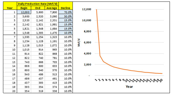
Figure #2: Percent Annual Decline
This method is good for a quick-and-dirty forecast, but it tends to yield overly optimistic annual volume numbers. That is because the annual decline rate is not a simple average of the beginning and end numbers. The decline rate tends to be higher in the first part of the year, and not quite so steep in the last part of the year. One obvious solution to this limitation is to do the same calculation as shown here, but do it on a monthly basis. While that does improve the accuracy of the curve estimation process, there is a much better alternative that can be used with the same input data.
Arps Curve Model
The Domino Effect Production Economics Model uses the Arps curve model introduced in Chapter 9 of The Domino Effect. This method was developed by mining engineer J. J. Arps in 1944. The method and numerous variants have been in general use by much of the oil and gas industry ever since. The Arps approach assumes that a well’s production profile can best be expressed mathematically by a curve belonging to the hyperbolic family of equations. Over the 70+ years since the Arps curve was introduced, it has proved to be an accurate way to model type curves, given some simple assumptions about the IP rate and production declines over time.
Figure #2 below is the Arps equation. Don’t panic. We will not go through the math of how this works. There are more than enough mathematical explanations that can be found by Googling Arps Decline Curve. For our purposes, all you really need to know is that the Arps equation is built into a macro in The Domino Effect Production Economics Model.
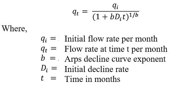
A key variable in the Arps equation is the Arps decline curve exponent, or b. This number basically tells the equation the shape of the curve. The Domino Effect Production Economics Model macro calculates this input variable, based on annual decline rate estimates in a format similar to the Percent Annual Decline input numbers shown in the blue cells, Figure #1. For more information on use of the model, go to http://thedominoeffect.com/prodecon.
The following important assumptions underlie the use of the Arps equation.
- Stable production at capacity: Arps curve analysis assumes that over the initial period of analysis the well is producing in a stable manner. In industry parlance, the well is producing at a constant “choke size” (a choke is the piece of equipment that restricts the diameter of the wellhead outlet) or at a constant wellhead pressure..
- Constant production mechanism: an assumption that the Arps curve is only valid if the production mechanism remains the same over the life of the well. This assumes no infill drilling, fluid injection, or additional fracturing takes place during the life of the well.
- Constant Flow State: The Arps curve assumes that the IP used excluded any extraordinary or volatile flows that may occur in the first few days of a well’s production.
Decline rate analysis incorporates equal parts of art and science. The art is in collection, summarization and estimation of the data to be used in the analysis. The science is in the process to calculate the decline curve values. Due to differences in data sources and assumptions, it is quite possible that two analysts using the exact same modeling process can come up with substantially different type curves, which will generate different rates of returns in the production economics calculations. Only by knowing the sources of the data, the assumptions made and the methodology used can you confidently interpret the production economics from any analyst.