
This Extra Content Segment is provided for readers of The Domino Effect that are not familiar with the concepts of discounted cash flows, internal rates of return or the math of time value of money. If you have an MBA degree, you probably want to skip this segment.
The Basics
A bird in the hand is worth two in the bush. That wise old maxim means that you would rather have a dollar in your hand today than the prospect -- but not the certainty – of getting two dollars later. That is pretty obvious, right? You may never see the two dollars, but the one dollar is already ‘in your hand’.
Consider a slightly different situation. What if you were equally assured of getting a dollar in your hand (no uncertainty about whether you’ll get the dollar or not), but your choice was to get that dollar today, or get the same dollar a year from now. Most of us would choose getting the dollar today. That way we can do what we want to do with the dollar. We can spend it. Or we could use that dollar to make a little more money – earning interest in a savings account (making not much money these days), investing in the stocks or bonds of a company, or (along with other dollars) investing in some kind of income earning asset.
Let’s make it a little more interesting. Instead of a dollar, say the amount is $10,000. You can receive the $10,000 today, or a year from now. Let’s also assume that you don’t need the money for some extravagant purchase or to repay Guido, your friendly loan shark. So you can get the money today and sock it away in some relatively safe investment, or wait a year and only then invest the money. If you took the money today and put the money to work in an investment earning 5% per year, at the end of the year you would have $10,500. Clearly taking the money today and investing it is better than waiting a year to get the $10,000, because you are $500 better off.
The difference between $10,000 for money that can be invested today and yield $10,500 in a year versus getting only $10,000 in a year is an example of the ‘time value of money’. The theory here is that money today is worth more than money in the future. Or said another way, the sooner you get money the better off you are. Because you can take money received sooner and do something else with it, like invest it to make still more money.
Comparing Investment Alternatives
The time value of money concept is fundamental to the financial analysis of alternative investments. You want to put your money into investments that return your money quicker, not just because you want to get money sooner, but because you can theoretically use the money you get back to invest in something else.
So let’s see how this works. Say you have two investment alternatives. Both require an investment of your $10,000 in the example above. Alternative A will get you $12,000 back after a year. Alternative B will get you $6,000 back after a year, and then another $6,500 the next year. So Alternative B is better, right? You get $12,500 instead of only $12,000. The answer is that it depends.
It depends on where the money comes from, and on what you plan to do with the money that you get back. There are all sorts of super-sophisticated financial models that MBAs use to get the answer to that question. When calculated for a company, they call that answer the company’s ‘Cost of Capital’. In other words, what does it cost you to get that $10,000 in the first place. Most likely somebody did not just hand you that $10,000 because you are nice person. You had to go out and raise that money somehow. For simplicity sake, let’s say you borrowed the money. And you had to pay a 10% annual rate of interest on the money. So your before tax cost of capital is 10%. (We are going to completely ignore taxes in this exercise – way too complicated for an introduction to DCF analysis.)
Before we get to the details of the calculations, let’s first look at the answer in Figure #1 below. In the spreadsheet table we show our $10,000 investment as a negative in year 0, meaning now. Then at the end of year 1, we receive $12,000 for Alternative A, and $6,000 for Alternative B. At the end of year 2 we get another $6,500 from Alternative B, nothing from Alternative A. So we get $500 more from B than A. But which is a better investment?
In this example we used the Excel function =NPV(). NPV stands for net present value, which is another term for discounted cash flow (DCF). We’ll show how the =NPV() math works later.
Applying a 10% discount rate in the formula, the answer for Alternative A comes out at $909, while B comes out at $826 (blue cells). So A wins on a DCF basis, even though Alternative B earns more total dollars. That is because getting the $12,000 back in a year is better than getting $6,000 back in a year but having to wait still another year to get the remaining $6,500. But here’s an interesting fact. If we use a discount rate of 5% for both investments, Alternative A comes out at $1,429, while B comes out at $1,610 (green cells). In this case, Alternative B wins. Why? Because getting the money back sooner is not as important if your borrowing rate is 5% versus if it is 10%. Your money costs you less, so from a financial perspective you are better off letting your money stay invested longer. As you might imagine, this math has had huge implications for the economy as a whole while the Federal Reserve has kept interest rates at rock bottom for the past few years.
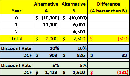
Figure #1: Alternative Investment Cases
The Math
You can’t really understand how this works unless you follow the math. So let’s look at the calculations if you didn’t use =NPV() but instead did the calculations the old fashioned way, with arithmetic. We’ll start with Alternative A. We invest the $10,000 now. So from today’s perspective, $10,000 is worth $10,000. Nothing tricky yet. But we don’t get the $12,000 for a year in the future. Not having that money for a year is a cost. And we know what that cost is – it is 10%, or cost of capital. So that $12,000 a year from now is worth less than $12,000. How much less? Well, it would be the amount of money we would need today to earn our 10% cost of capital on that $12,000. There is an easy way to calculate that number. Just divide $12,000 by the number one, plus the discount rate (i.e, the cost of capital). So the formula is 12,000 / (1 +.10) = 10,909. Don’t believe it? Say you have $10,909 today and earn 10% on it. 10,909 * .10 = 1,091. Add 1,091 to 10,909 and what do you get? That’s right. $12,000.
So if we take the discounted value of what we get back after a year which is $10,909 and subtract what we invested in the first place, the $10,000. We get the discounted cash flow answer, $909. In the 5% case the formula is 12,000 / (1 +.05) = 11,429. Like last time we subtract what we invested in the first place and get the discounted cash flow answer, $1,429. Note that the lower discount rate makes a big difference to the answer. Obviously you want to borrow money for the lowest possible rate.
That is all well and good for Alternative A, but in Alternative B we don’t get that last $6,500 for two years. You’ve already figured out that money not received for two years is worth less today than money received after only one year, right?. But how does that math work. Unfortunately we have to get into a little higher math, and that is exponents. Since it will be two years before we get our money, we are looking for the amount today that if we invested at our discount rate for two years would equal $6,500. That formula is 6,500 / (1 + .10)^2. In other words, we are going to multiply our interest rate term by itself before doing the division. If it were three years, we would use an exponent of ^3, four years ^4. So the further out you go you are dividing by a bigger number, which means the answer gets smaller. Which makes sense. The further out the money is, the less it is worth to you today.
So now to get the answer for Alternative B, we need to calculate the discounted cash flow for $6,000 at the end of year 1 and $6,500 at the end of year 2, then subtract the $10,000 investment. (6,000 / (1+.10)) + (6,500 / (1+.10)^2) -10000) = $826. Work through the numbers until you understand the math. Then never do it again. Because it is so much easier to use the Excel =NPV() function that you would be nuts to ever use this math in real life.
The Implications for Oil and Gas Producers
Here’s the bottom line for oil and gas producers. Shale wells tend to have big IP rates and steep decline curves. That may sound bad, but it is actually good. Because those high IP rates get producers their money back much quicker than conventional wells. Even though the decline rates are steep, the high IP rates tend to make up for it. Because those high IP rates imply that there is a lot of cash coming back to the producer just as soon as the well comes online. It is that money coming back quickly that makes the NPVs on shale wells look so good, and is one important reason why so much drilling is still going on at the low prices we see in the market today.